Markov Chain — Birth-Death Processes

Posted on December 11, 2014 by admin

– Stochastic Course Notes

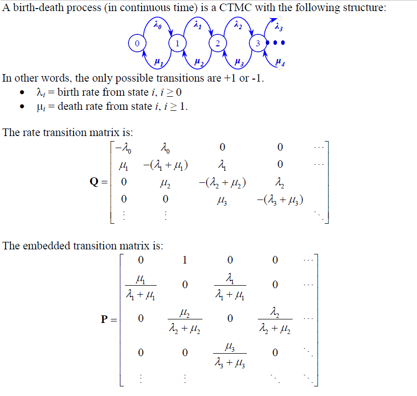
1. Definition

2. Expected Time to State n

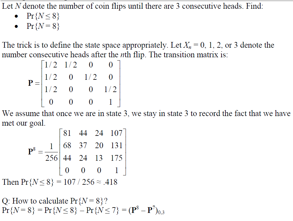
3. Example

Markov Chain — Branching Process

Posted on December 11, 2014 by admin

– Stochastic Course Notes

1. Definition

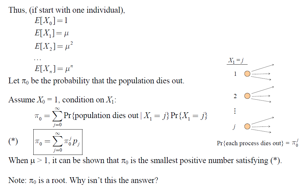
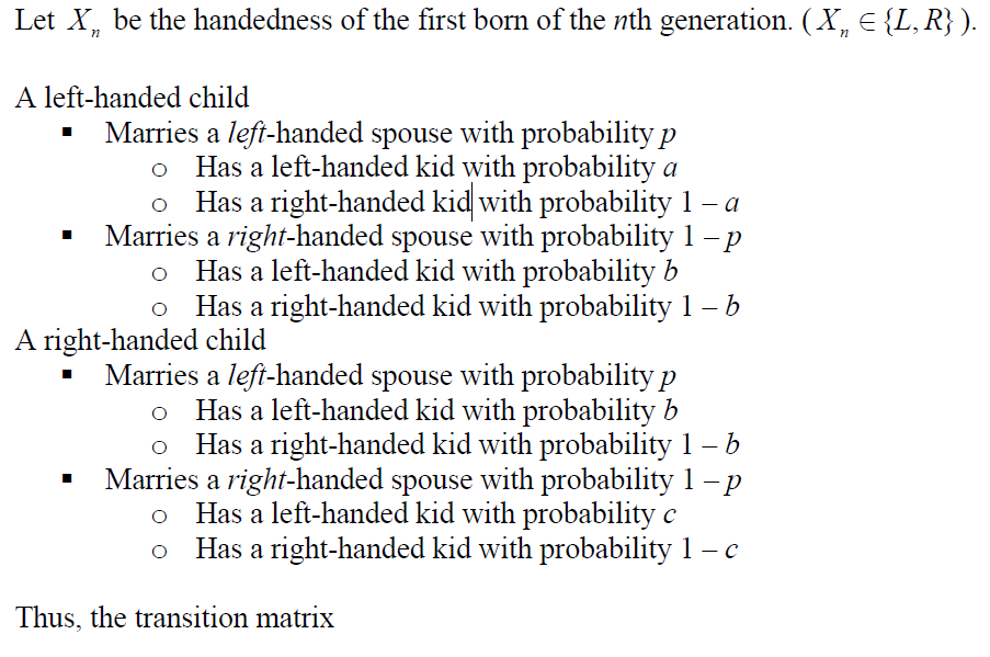
Consider a population

Each individual produces j new offspring each period with probability $p_j, j geq 0$ . Key assumption: This distribution is constant over time.
Assume that $p_j < q$ for all j (i.e., the problem is not deterministic)
Let $X_n$ be the size of the population at period n

2. Number of Population in the n-th Generation

3. Probability of Die Out

Analysis

Example

4. Example: Family Genetics

Problem:

Solution:

Markov Chain — Tendem Queue

Posted on December 11, 2014 by admin

– Stochastic Process Course Notes

1. Example: Tendem Queue

Problem:

Solution:

Markov Chain – Classifications of States

Posted on December 11, 2014 by admin

1. Definition of States

Communicate: State i and j communicate ( $i leftrightarrow j$ ) if i is reachable from j and j is reachable from i. (Note: a state i always communicates with iteself)
Irreducible: a Markov chains is irreducible if all states are in the same communication class.
Absorbing state: $p_(ii) = 1$
Closed Set: a set of states S is a closed set if no state outside of S is reachable from any state in S. (This is like absorbing set of states)
$f_i$ : be the probability that, starting in state i, the process returns (at some point) to the sate i
Transient: a state is transient if $f_i < 1$
Recurrent: a state that is not transient is recurrent, i.e., $f_i =1$ . There are two types of reurrent states

Positive recurrent: if the expected time to return to the state if finite
Null recurrent: if the expected time to return to the sate i is infinite (this requires an infinite number of states)

Periodic: a state is i period if $k>1$ where k is the smallest number such that all paths leading from state i back to state i has a multiple of k transitions
Aperiodic: if it has period k =1
Ergodic: a state is ergodic if it is positive recurrent and aperiodic.

2. Example: Gambler’s Ruin

3. Example: Random Walk

Markov Chain (Continuous Time)

Posted on December 11, 2014 by admin

1. Definition

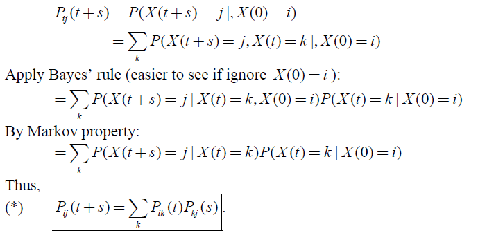
t-step transition probability: Let $P_{ij}(t)$ be the probability that the system is in state j in t time units, given the system is in state i now.

$P_{ij}(t) = P(X(t+s) = j | X(s) = i)$
= $P(X(t) =j | X(0) = i)$ (by stationarity)

2. Properties

Lemma 6.2 $lim_{t to 0} frac{1-P_{ii}(h)}{h} = v_i$

Lemma 6.2 b: $lim_{h to 0} = frac{P_{ij}(h)}{h} = q_{ij} = v_i p_{ij}$

Lemma 6.3:

3. Forward Chapman-Kolmogorov Equations

$P'_{ij}(t) = sum_{k neq j} q_{kj} P_{ik}(t) - v_j P_{ij}(t)$

Proof:

Define $q_{jj} = -v_j$

Markov Chain (Discrete Time)

Posted on December 11, 2014 by admin

1. Definition

Let ${X_n, n =0,1,cdots}$ be a stochastic process, taking on a finite or countable number of values.

$X_n$ is a DTMC if it has the Markov property: Given the present, the future is independent of the past
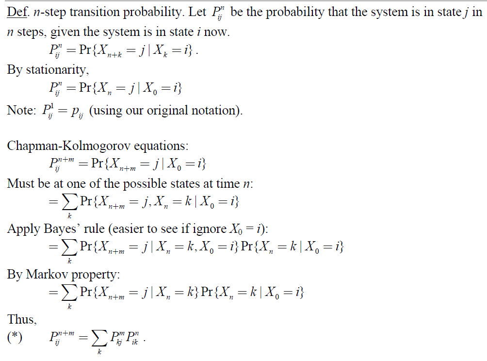
$P{X_{n+1} = j| X_n = j, X_{n-1} = i_{n-1} ,cdots, X_1 = i_1, X_0 = i_0} = Pr{X_{n+1} = j| X_n = i}$

We define $Pr{X_{n+1} = j| X_n = i} = P_{ij}$ , since $X_n$ has the stationary transition probabilities, this probability is not depend on n.

Transition probabilities satisfy $sum_j p_{ij} = 1$

2. n Step transition Probabilities

$P^{n+m}_{ij} = sum_k p^m_{kj} p^n_{ik}$

Proof:

3. Example: Coin Flips

4. Limiting Probabilities

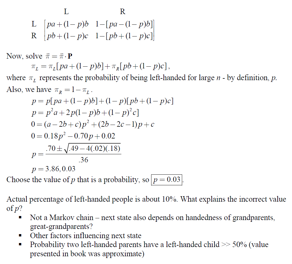
Theorem: For an irreducible, ergodic Markov Chain, $pi_j = lim_{n to infty} P^n_{ij}$ exists and is independent of the starting state i. Then $pi_j$ is the unique solution of $pi_j = sum_i pi_i P_{ij}$ and $sum_j pi_j = 1$ .

Two interpretation for $pi_i$

The probability of being in state i a long time into the future (large n)
The long-run fraction of time in state i

Note:

If Markov Chain is irreducible and ergodic, then interpretation 1 and 2 are equivalent
Otherwise, $pi_i$ is still the solution to $pi = pi P$ , but only interpretation 2 is valid.

Splitting a Poisson Process: M/G/Infinity Queue

Posted on December 11, 2014 by admin

1. Notation

M: “Markovian” or “Memoryless” arrival process (i.e., Poisson Process)
G: General service time (not necessarily exponential)
$infty$ : Infinite number of servers

Let

$X(t)$ be the number of customers who have completed service by time t
$Y(t)$ be the number of customers who are being served at time t
$N(t)$ be the total number of customers who have arrived by time t

2. Splitting the arrival process

Fix a reference time T.
Consider the process of customers arriving prior to time T.
A customer arriving at time $t leq T$ is

Type I: if service is completed before T

occur with probability $P_i(t) = G(T-t)$

Type-II: if customer still is service at time T

occur with probability $P_{II}(t) = G^c(T-t)$

Since arrival times and services times are all independent, the type assignments are independent. Therefore,

$X(T)$ is a Poisson random variable with mean $lambda int^T_0 P_I(t) dt = lambda int^T_0 G(T-t) dt = lambda int^T_0 G(t)dt$ .
$Y(T)$ is a Poisson random variable with mean $lambda int^T_0 P_{II}(t)dt = lambda int^T_0 G^c(T-t)dt = lambda int^T_0 G^c(t)dt$
$X(T)$ and $Y(T)$ are independent

What happens when $T to infty$

$G(t) approx 1$ for large t. Therefore, $X(T)$ is a Poisson random variable with mean $lambda t$
$Y(T)$ is a Poisson random variable with mean $lambda int^T_0 G^ct)dt = lambda E[G]$

Summary: Number of customers in service in an $M/G/infty$ queue, in steady state, is a Poisson random variable with mean $lambda E[G]$ .

3. Example

Compound Poisson Process (CPP)

Posted on December 11, 2014 by admin

1. Definition:

Remove the restriction that two or more customers cannot arrive at the same time, (i.e., remove orderliness property)

Let $N(t)$ be a Poisson Process with rate $lambda$ , and let $Y_i$ be the i.i.d random variable, then $X(t) = sum^{N(t)}_{i=1} Y_i$ is a compound Poisson process

Example #1: Buses arrive according to a Poisson process. Let $Y_i$ be the number of people on bus i, and let $X(t)$ be the total number of people arriving by time t.

Example #2: Insurance claims arrive according to a Poisson process. Let $Y_i$ be the size of the claim (in dollars), and let $X(t)$ be the total amount due to all claims by time t.

2. Expectation:

$E[X(t)] = E[E[X(t)|N(t)]]$

Since $E[X(t)|N(t) = n] = E[sum^n_{i=1} Y_i] = nE[Y_i]$ , i.e., $E[X(t)|N(t)] = N(t)E[Y_i]$

So $E[E[X(t)|N(t)]] = E[N(t)E[Y_i]] = E[N(t)]*E[Y_i] = lambda t E[Y_i]$

3. Variance:

var[X(t)] = var[E[X(t)|N(t)]] + E[var[X(t)|N(t)]]

and we have $Var[X(t)|N(t)=n] = var(sum^n_{i=1} E[Y_i]) = nVar[Y_i]$
or $var(X(t)|N(t)) = N(t)Var(Y_i)$ .
So $Var[E[X(t)|N(t)]] + E[Var[X(t)|N(t)]]$
= $Var[N(t)E(Y_i)] + E[N(t)Var[Y_i)]$
= $lambda t E^2[Y_i] + lambda t Var(Y_i)$
= $lambda t E^2[Y_i] + lambda t (E[(Y_i)^2] - E^2[Y_i])$
= $lambda t E[(Y_i)^2]$

4. Example:

Non-Homogeneous Poisson Process (NPHH)

Posted on December 11, 2014 by admin

1. Properties:

N(0) = 0
N(t) has independent increments
$Pr{N(t+h) - N(t)} = lambda(t)h + o(h)$
$Pr{N(t+h)-N(t) geq 2} = o(h)$

Notes:

This is like a Poisson process, without the stationary assumption

A process with the above properties is a NHPP with intensity (or rate) function $lambda(t)$

2. Definition:

The mean value function (for a NHPP) is

$m(t) = int^t_0 lambda(u) du$

3. Key Properties:

For a NHPP, N(s+t) – N(s) is a Poisson random variable with mean $m(s+t) - m(s)$

The Poisson Process

Posted on December 11, 2014 by admin

1. Priliminary Definitions

Def : A stochastic process is a collection of random variable (RV) indexed by time ${X(t), t in T}$ .

If T is continuous set, the process is a continuous time stochastic process (e.g., Poisson Process)
If T is countable, then the process is a discrete time stochastic process (e.g., Markov chain)

Def. A counting process is a stochastic process ${N(t); t geq 0}$ such that

$N(t) in {0,1,cdots, 2}$ (that is, N(t) is non-negative integer)
If $s < t$ , the $N(s) leq N(t)$ ( that is, N(t) is non-decreasing in t)
For $s<t$ , $N(t) - N(s)$ is the number of events occurring in the time interval $(s,t]$ .

Def: A counting process has stationary increments if the distribution of the number of events in an interval depends on the length of the interval, but not on the starting point of the interval. That is, $P(N(s+t) - N(s) = n)$ does not depend on s. Intuitively, the interval can be “slide” around without changing its stochastic nature.

2. Definition of Poisson Process

Definition 1: A Poisson process is a counting process ${N(t); t geq 0}$ with rate $lambda >0$ , if:

N(0) = 0;
The Process has independent increments
The number of events in any interval of length t is a Poisson RV with mean $lambda t$ .

That is, for all $s,t geq 0$ and $n = 0,1,2, cdots$

$P(N(s+t) - N(s) = n) = e^{-lambda t} (lambda t)^{n}/n!$ .

Definition 2: A Poisson process is a counting process ${N(t); t geq 0}$ with rate $lambda >0$ if

N(0) = 0
The process has stationary increments
The process has independent increments
$Pr{N(h) =1} = lambda h + o(h)$ (# of events approximately proportional to the length of interval)
$Pr{N(h) geq 2} = o(h)$ (can’t have 2 or more events at the same time — “orderliness”)

Eliminating of individual assumptions yields variations on the Poisson process

Eliminate assumption 2, Non-stationary Poisson Process
Eliminate assumption 3, Mixture of Poisson Process (choose $lambda$ randomly, then run a Poisson process)
Eliminate assumption 5, compound Poisson Process

Definition 3: A Poisson process with rate $lambda$ is a counting process such that times between events are i.i.d distribution exp( $lambda$ )

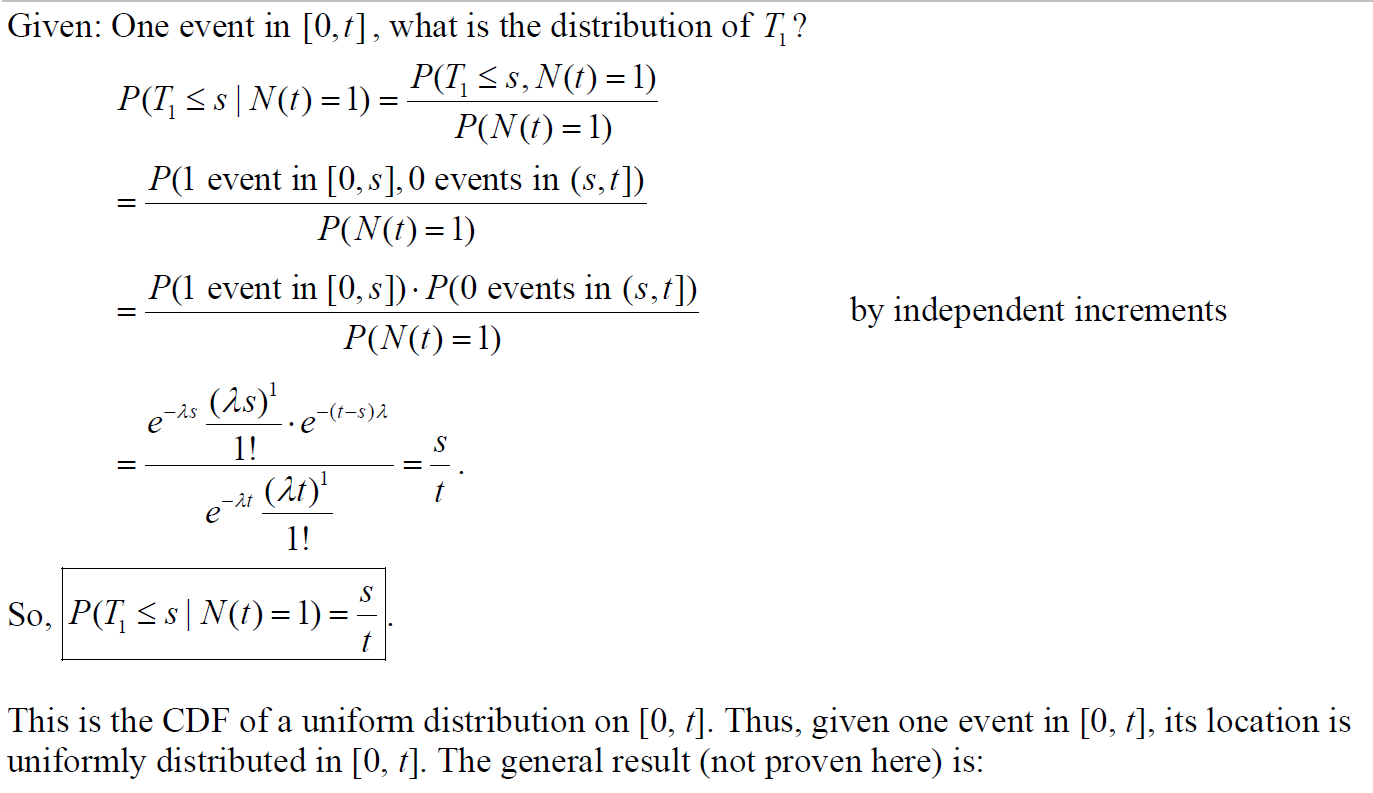
3. Conditional Distribution of Event Times