Process Stack

Stacks usually grown down, i.e., the stack starts at a higher address in memory and progressively gets lower.

Stack Pointer

  • To keep track of current growth of the stack, the hardware defines a register as the stack pointer. 
  • The compiler (or the programmer, when writing in assembler) users this register to keep track of current top of the stack. 
  • Store
    • It is stored in the register ESP.

Call Stack

  • A call stack is used for several related purposes, but the main reason for have one is to keep track of the point to which each active subrountine should return control when it finishes executing.
  • Active subrountine
    • An active subrountine is one that has been called by yet to complete execution after which control should be handed back to the point of the call. 

How it works?

  • Return address
    • Store the returning address somewhere, so that we can continue executing the current function after completion of called function.
  • Other info
    • Saving other information about current function. 
  • Parameters
    • Providing the callee with the parameters
  • Provided called function some space to store its automic variables
  • Return value
    • Providing some mechanism to get return value from the called function. 
    • It is implemented using EAX register. Called function stores return value in EAX.

Execution in Steps

  1. Push the parameters in the reverse order (right to left)
  2. Call function now
    1. It implicitly pushes the return address into STACK
  3. Push the current EBP
    1. i.e., push Frame Pointer (FP) of calling function into stack. We need to do this to continue with the execution of calling function after return from the called function,
  4. Copy the ESP to EBP
    1. Yes, this location will be the new FRAME Pointer
  5. Allocate space on stack for local variable
    1. It is done by decrementing ESP
  6. Put the value to be returned in EAX
  7. Copy current EBP to ESP
    1. It will reduce stack size. Now we have the old FP at the top of the stack??

Stack Frame

  • The stack frame generally includes the following components
    • The return address
    • Argument variables passed on the stack
    • Local variables
    • Saved copies of any registers modified by the subprogram that need to be restored.

Stack Overflow

  • Introduction
  • Suggestion
    • If you are a programmer accept arbitrary input into a stack variable (say, reading from the keyboard or over the network), you need to say how big that data is going to be
    • OS
      • The OS can make the stack not executable. 

Reference

[1] http://articles.manugarg.com/stack.html

Process Communication

Shared Memory Systems

  • In general, the memory to be shared in a shared-memory system is initially within the address space of a particular process, which needs to make system calls in order to make that memory publicly available to one or more other processes. 
  • Other processes which wish to use the shared memory must then make their own system calls to attach the shared memory area onto their address space. 
  • Generally a few messages must be passed back and forth between the cooperating processes first in order to set up and coordinate the shared memory access. 

Example” POSIX Shared Memory

  • Step 1: one of the processes involved to allocate some shared memory, using shmget
    • int segment_id = shmget(IPC_PRIVATE, size, S_IRUSR | S_IWUSR)
      • The first parameter 
        • specifies the key (identifier) of the segement. IPC_PRIVATE creates a new shared memory segment.
      • The second parameter
        • How big the shared memory segment is to be, in bytes.
      • The third parameter
        • A set of bitwise ORed flags. In this case, the segment is being created for reading and writing.
      • The return value
        • an integer identifier
  • Step 2: Any process which wishes to use the shared memory must attach the sahred memory to their address space, using shmat
    • char* shared_memory = (char *) shmat(segment_id, NILL, 0)
      • The first parameter
        • Specify the key of the segment that the process wishes to attack to its address space
      • The second parameter
        • Indicate where the process wishes to have the segment attacked. Null insicates the system should decide.
      • The third parameter
        • A flag for read-only operation. Zero indicates read-write; One indiciates Readonly.
      • The return value
        • The return value of shmat is a void *, which the process can use (type cast) as appropriae. In this example, it is being used as a character pointer. 
  • Step 3: The process may access the memory using the pointer returned by shmat. For example, using sprintf
    • sprintf(shared_memory, “Writing to shared memoryn”);
  • Step 4: When a process no longer needs a piece of shared memory, it can be detached using shmtd
    • shmat(shared_memory)
  • Step 5: And finally the process that originally allocated the shared memory can remove it from the system using shmctl.
    • shmctl(segment_id, IPC_RMID)

Message-Passing

  • Message passing systems must support at a minimum system calls for “send message” and “receive message”
  • A communication link must be established between the corresponding process before message can be sent. 
  • There are three key issues to be resolved in message passing systems
    • Direct or indirect communication (naming)
    • Synchronous or asynchronous communication
    • Automatic or explicit buffering

Naming

  • Direct communication
    • With direct communication the sender must know the name of the receiver to which it wishes to send message
  • Indirect communication
    • Multiple processes can share the same mailbox or boxes.
    • Only one process can read any given message in a mailbox. 
    • The OS must provide system calls to create and delete mailboxes, and to send and receive messages to/from mailboxes.

Synchronization

  • Either the sending or receiving of messages (or neither or both) may be either blocking or non-blocking.

Buffering

  • Messages are passed via queues, which may have one or three capacity configurations
    • Zero capacity
      • Message cannot be stored in the queue, so senders must lock until receivers accept the messages.
    • Bounded capacity
      • There is a certain pre-determined finite capacity in the queue. Senders must block if the queue if full, until space becomes available in the queue, but may be either blocking or non-blocking otherwise. 
    • Unbounded capacity
      • The queue has a theoretical infinite capacity, so senders are never forced to block. 

Reference

[1] https://www.cs.uic.edu/~jbell/CourseNotes/OperatingSystems/3_Processes.html

Process Memory, State, and Scheduling

Process Concept

  • A process is an instance of a program in execution

Process Memory

  • Text: 
    • comprises the compiled program code, read in from non-volatile storage when the program is launched. 
  • Data
    • Stores global and static variables, allocated and initialized prior to executing main.
  • Heap
    • Used for dynamic memory allocation, is managed via calls to new, delete, malloc, free etc. 
  • Stack
    • Used for local variables
    • Space on the stack is reserved for local variables when they are declared (at function entrance or elsewhere, depending on the language), and the space is freed up when the variables go out of scope
    • The stack is also used for function return values, and the exact mechanisms for stack management may be language specific. 
  • When processes are swapped out of memory and later restored, additional information must also be stored and restored. Key among them are the program counter and the value of all program registers

Process State

  • New
    • The process is in the stage of being created.
  • Ready
    • The process has all the resources available that it needs to run, but the CPU is not currently working on this process’s instruction.
  • Running
    • The CPU is working on this process’s instruction.
  • Waiting
    • The process cannot run at the moment, because it is waiting for some resource to become available for some event to occur. For example, the process may be waiting for keyboard input, disk access request, inter-process messages, a time to go off, or a child process to finish.
  • Terminated
    • The process has completed.

Process Control Block

For each process, there is a Process Control Block (PCB), which stores the following (types of) process-specific information.
  • Process State
    • Running, waiting etc. 
  • Process ID
    • and also parent process ID
  • CPU registers and Program Counter
    • These need to be saved to restored when swapping processes in and out of the CPU
  • CPU scheduling information
    • Such as priority information and pointers to scheduling queues
  • Memory-Management information
    • e.g., page tables or segment tables
  • Accounting information
    • User and kernel CPU time consumed, account numbers, limits, etc. 
  • I/O Status information
    • Devices allocated, open file tables etc. 

Process Scheduling

  • The two main objectives of the process scheduling system are to keep the CPu busy at all times and to deliver “acceptable” response times for all program, particularly for interactive ones. 
  • The process scheduler must meet these objectives by implementing suitable policies for swapping process in and out of the CPU.

Scheduling Queues

  • Job queue
    • All processes are stored in the job queue.
  • Ready queue
    • Processes in the Ready state are placed in the ready queue
  • Device queue
    • Processes waiting for a device to be available or to deliver data are placed on device queues. There is generally a separate device queue for each device.

Scheduler

  • Long-term scheduler
    • Typically of a batch system or a very heavily loaded system. It runs infrequently, (such as when one process ends selecting one or more to be loaded in from disk in its place), and can afford to take the time to implement intelligent and advanced scheduling algorithms
  • Short-term scheduler, or CPU scheduler
    • Runs very frequently, on the order of 100 milliseconds, and must very quickly swap one process out of the CPU and swap in another one.
  • Medium-term scheduler
    • Some systems also employ medium-term scheduler.
    • When system loads get high, this scheduler will swap one or more processes out of the ready queue system for a few seconds, in order to allow smaller faster jobs to finish up quickly and clear the system. 

    Reference

    [1] https://www.cs.uic.edu/~jbell/CourseNotes/OperatingSystems/3_Processes.html

    Introduction to Memory

    1. Background

    • Program must be brought (from disk) to memory and placed within process for it to be run
    • Main memory and registers are only storage CPU can access directly
    • Memory unit only sees a stream of addresses + read requests
      • or address +data and write request
    • Register access in one CPU clock (or less)
    • Main memory can take many cycles (stalls)
    • Cache sit between main memory and CPU registers
    • Protection of memory required to ensure correct operation 
    2. Address binding
    • Addresses represented in different ways at different stages of a program’s life
      • source code addresses usually symbolic
      • compile code addresses bind to relocated addresses
        • i.e., 14 bytes from beginning of this module
      • Linker or loader will bind relocatable addresses to absolute addresses
      • Each binding maps one address space to another
    • Address binding of instructions and data to memory addresses can happen at three different stages
      • compile time: if memory location known a priori, absolute code can be generated; must recompile code if starting location changes
      • load time: must generate relocatable code if memory location is not known at compile time
      • execution time: binding delayed until run time if the process can be moved during its execution from one memory segment to another
        • need hardware support for address maps (e..g, base and limit registers)
    3. Multistep Processing of a user program
    4. Logical v.s. Physical Address Space
    • The concept of a logical address space that is bound to a separate physical address space is central to proper memory management
      • logical address: generated by the CPU; also referred to as virtual address
      • physical address: address seen by the memory unit
    • Logical and physical addresses are the same in compile-time and load-time address-binding schemes; logical (virtual) and physical addresses differ in execution-time address-binding scheme.
    • Logical address space is the set of all logical addresses generated by a program
    • Physical address space is the set of all physical addresses generated by a program
    5. Dynamic loading
    • routine is not loaded until it is called
    • better memory-space utilization; unused routine is never loaded
    • all routines kept on disk is relocatable load format
    • useful when large amounts of code are needed to handle infrequently occurring cases
    • no special support from the operation system is required
      • implemented through program design
      • OS can help by providing libraries to implement dynamic loading
    6. Dynamic Linking
    • Static linking
      • system libraries and program code combined by the loader into the binary program image
    • Dynamic liking
      • linking postponed until execution time
        • small piece of code, stub, used to locate the appropriate memory-resident library rountine
    • Stub replaces itself with the address of the routine, and executes the routine
    • Operating system checks if routine is in processes’ memory address
      • if not in address space, add to address space
    • Dynamic linking is particularly useful for libraries
      • system also known as shared libraries
    • Consider applicability to patching system libraries
      • versioning may be needed
    7. Base and Limit Registers
    • A pair of base and limit registers define the logical address space
    8. Hardware address protection with base and limit registers
    9. Memory Management Unit (MMU)
    • Hardware device that at run time maps virtual to physical address
    • The user program deals with logical address; it never sees the real physical addresses
      • execution-time binding occurs when reference is made to location in memory
      • logical address bound to physical address

    10. Dynamic relocation using a relocation register

    Job Scheduling

    1. Objective

    • maximum CPU utilization obtained with multiprogramming
    • CPU-I/O Burst Cycle- Process execution consist of a cycle of CPU execution and I/O wait
    2. CPU Scheduler
    • Selects from among the processes in ready queue, and allocates the CPU to one of them
      • queues may be ordered in various ways
    • CPU scheduling decisions may take place when a process
      • switches from running to waiting sate
      • switches from running to ready state
      • switches from waiting to ready state
      • terminate
    • scheduling under 1 and 4 is non-preemptive
    • all other scheduling is preemptive
      • consider access to shared data
      • consider preemption while in kernel mode
      • consider interrupts occurring during crucial OS activicites
    3. Dispatcher
    • Dispacher module gives control of the CPU to the process selected by the short-term scheduler; this involves
      • switching context
      • switching to user mode
      • jumping to the proper location in the user program to restart that program
    • Dispatch latency
      • time it takes for the dispatcher to stop one process and start another running
    4. Scheduling Criteria
    • CPU utilization
      • keep the CPU as busy as possible
    • Throughput 
      • # of processes that complete their execution per time unit
    • Turnaround time
      • amount of time to execute a particular process
    • Waiting time
      • amount of time a process has been waiting in the ready queue

    5. First-Come. First-Server (FCFS) Scheduling

    6. Shortest-Job-First (SJF) Scheduling

    • associate with each process the length of its next CPU burst
      • use these lengths to schedule the process with the shortest time
    • SJF is optimal
      • gives minimum average waiting time for a given set of processes
        • the difficult is knowing the length of the next CPU request
    7. Determine the length of next CPU burst
    • can only estimate the length
      • should be similar to the previous one
      • then pick process with shortest predicted next CPU burst
    • can be done by using the length of previous CPU bursts, using exponential averaging
      • t_n = average length of the n-th CPU burst
      • tau_{n+1} = predicted value of the next CPU burst
      • alpha, 0 leq alpha leq (1-alpha) tau_n
    • commonly, alpha set to 1/2
    • preemptive version called shortest-remaining-time-first
    8. Example of Exponential Averaging
    • alpha = 0
      • tau_{n+1} = tau_n
      • recent history does not count
    • alpha = 1
      • tau_{n+1} = n tau_n
      • only the actual last CPU burst counts
    • If we expand the formula, we get
      • tau_{n+1} = alpha tau_n + (1-alpha) tau_{n-1} + ...
      •                     = (1-alpha)^j alpha tau_{n-j} + ...
      •                     = (1-alpha)^{n+1} tau_0
    • since both alpha and 1-alpha are less than or equal to 1, each successive term has less weight than its predecessor
    9. Example of Shortest Remaining-time-first

    10. Priority Scheduling
    • A priority number (integer) is associated with each process
    • The CPU is allocated to the process with the highest priority (smaller integer = highest priority)
      • preemptive
      • non-preemptive
    • SJF is priority scheduling where priority is the inverse of predicted next CPU burst time
    • Problem = starvation 
      • low priority processes may never execute
    • Solution = aging
      • as time progresses, increase the priority of the process
    11. Round Robin
    • Each process gets a small unit of CPU time (time quantum q), usually 10-100 milliseconds.
      • after this time has elapsed, the process is preempted and added to the end of the ready queue
    • If there are n processes in the ready queue and the time quantum is q, then each process gets 1/n of the CPU time is chunks of at most q time units at once. 
      • No process waits more than (n-1)q time units.
    • Time interrupts every quantum to schedule next process
    • Performance
      • q large : FIFO
      • q small: q must be large with respect to context switch, otherwise, overhead is too high
    • Example of Round robin with time Quantum =4 
    12. Multilevel Queue
    • Ready queue is partitioned into separate queues, e..g,
      • forground (iterative)
      • background (batch)
    • Process permanently in a given queue
    • Each queue has its own scheduling algorithm
      • forground-RR
      • background-FCFR
    • Scheduling must be done between the queues
      • fixed priority scheduling: i.e., serve all from foreground then from background
        • possibility starvation
      • time slices: each queue gets a certain amount of CPU time which it can schedule amongst its processes, i.e., 80% to foreground in RR
      • 20% to background in FCFS

    13. Multi-level feedback queue
    • a process can move between the various queues;
    • aging can be implemented this way
    • multi-level-feedback-queue scheduler defined by the following parameters
      • number of queues
      • scheduling algorithms for each queue
      • method used to determine when to upgrade a process
      • method used to determine when to demote a process
      • method used to determine which queue a process will enter when that process needs service
    • Example of multilevel feedback queue
      • three queues
        • Q_0: time quantum 8 milliseconds
        • Q_1: time quantum 16 milliseconds
        • Q_2; FCFS
      • scheduling
        • a new job enters queue Q_0 which is served FCFS
          • when it gains CPU, job received 8 milliseconds
          • if it does not finish in 8 milliseconds, job is moved to queue Q_1
      • at Q_1 job is again served FCFS and receives 16 additional milliseconds
        • if it still does not complete, it is preempted and moved to queue Q_2
    14. Thread Scheduling
    • Distinction between user-level and kernel-level threads
    • when threads supported, threads scheduled, not processes
    • many-to-one and many-to-many methods, thread library schedules user-level threads to run on LWP
      • known as process-contention scope (PCS) since scheduling competition is within the process
      • typically thread scheduled onto available CPU is system contention scope (SCS)
        • competition among all threads in the system
    15. Multi-Processor Scheduling
    • CPU scheduling more complex when multiple CPUs are available
    • Homogeneous processors within a multiprocessor
    • Asymetric multiprocessing
      • only one processor accesses the system data structures, alleviating the need for data sharing
    • Symmetric multiprocessing (SMP)
      • each processor is self-scheduling, all processes in common ready queue
      • or each has its own private queue of ready processes
    • Processor Affinity
      • process has affinity for processor on which it is currently running
        • soft affinity
        • hard affinity
        • variation including processor sets
    16. Multiplecore Processor
    • recent trend to place multiple processor cores on the same physical chip
    • faster and consumes lees power 
    • multiple threads per core also growing
      • takes advantage of memory stall to make progress on another thread while memory retrieve happens

    Monitor

    1. Monitor

    • high-level synchronization construct that allows the safe-sharing of an abstract data type among concurrent processes
    monitor monitor-name{
        shared variable declarations
        procedure body p1(){}
        procedure body p2() {}
        procedure body pn() {}
        {
            initialization code
        }
    }
    2. Schematic View of a Monitor

    • the monitor construct ensures that at most one process can be active within the monitor at a given time
    • shred data (local variables) of the monitor can be accessed only by local procedure

    3. Monitors Introduction

    • to allow a process to wait within the monitor
      • a condition variable must be declared, as condition x, y
    • condition variable can only be used with the operation wait and signal
      • the operation 
        • x.wait() means that the process invoking this operation is suspended until another process invokes x..signal()
        • x.signal() operation resumes exactly one suspend process on condition variable x. If no process is suspended on condition variable x, then the signal operation has no effect.
        • wait and signal operations of the monitors are not the same as semaphore wait and signal operations
    4. Monitor with condition variables
    • when a process P signal to wake up process Q that was waiting on a condition, potentially both of them can be active.
    • however, monitor rules require that at most one process can be active within the monitor
      • signal and wait: P waits until Q leaves the monitor
      • signal and continue: Q waits until P leaves the monitor (or, until P waits for another condition)
      • Signal and leave: P has to leave the monitor after signaling
    • the design decision is different for different programming languages
    5. Procedure-Consumer Problem With Monitor

    6. Dining-Phisolophers Problem with Monitors

    Process Synchronization

    1. Concurrent access to shared data

    • Example
      • suppose that two processes A and B have access to a shared variable “Balance”
        • process A: Balance = Balance – 100
        • process B: Balance = Balance – 200
      • Further, assume that Process A and Process B are executing concurrently in a time-shared, multiprogrammed system
      • The statement “balance = balance – 100” is implemented by several machine level instructions such as
        • A1. LOAD R1, BALANCE //load BALANCE from memory to register 1 (R1)
        • A2. SUB R1, 100 //subtract 100 from R1
        • A2. STORE BALANCE, R1 //store R1’s contents back to the memory location of BALANCE
      • Similarly, “BALANCE = BALANCE – 200” can be implemented in the following
        • B1. LOAD R1, BALANCE
        • B2. SUB R1, 200
        • B3. STORE BALANCE, R1
    2. Race Condition
    • Observe: in a time-shared system, the exact instruction execution order cannot be predicted
    • Situations like this, where multiple processes are writing or reading some shared data and the final result depends on who runs precisely when, are called race conditions.
    • A serious problem for any concurrent system using shared variables.
    • We must make sure that some high-level code sections are executed atomically.
    • Atomic operation means that it completes in its entirety without worrying about interruption by an other potentially conflict-causing process.
    3. The Critical-Section Problem
    • n processes are competing to use some shared data
    • Each process has a code segment, called critical section (critical region), in which the shared data is accessed.
    • Problem: ensure that when one process is executing in its critical section, no other process is allowed to execute in that critical section.
    • The execution of the critical sections by the processes must be mutually exclusive in time
    4. Solving Critical-Section Problem
    Any solution to the problem must satisfy four conditions
    • Mutual Exclusion
      • no two processes may be simultaneously inside the same critical section
    • Bounded Waiting
      • no process should have to wait forever to enter a critical section
    • Progress
      • no process executing a code segment unrelated to a given critical section can block  another process trying to enter the same crtical section
    • Arbitrary speed
      • no assumption can be made about the relative speed of different processes (though all processes have a non-zero speed)
    5. General Structure of a Typical Process
    do{
    entry section
         critical section
    exit section
         remainder section
    } while(1);
    • we assume this structure when evaluating possible solutions to Critical Section Problem
    • in the entry section, the process requests “permission”
    • we consider single-processor systems
    5. Getting help from hardware
    • one solution supported by hardware may be to use interrupt capability
    do{
         DISABLE INTERRUPTS
              critical section;
         ENABLE INTERRUPTS
             remainder section
    } while(1);
    6. Synchronization Hardware
    • Many machines provide special hardware instructions that help to achieve mutual exclusion
    • The TestAndSet (TAS) instruction tests and modifies the content of a memory word automatically
    • TAS R1, LOCK
      • reads the contents of the memory workd LOCK into register R!
      • and stores a nonzero value (e.g. 1) at the memory word LOCK (again, automatically)
        • assume LOCK = 0;
        • calling TAS R1, LOCK will set R! to 0, and set LOCK to 1
        • Assume lOCK = 1
        • calling TAS R1 LOCK will set R1 to 1, and set LOCK to 1
    7. Mutual Exclusion with Test-and-Set
    • Initially, share memory word LOCK = 0;
    • Process pi
    do{
         entry-section:
          TAS R1, LOCK
          CMP R1, #0
          JNE entry_section //if not equal, jump to entry
             critical section
          MOVE LOCK, #0 //exit section
             remainder section
    } while(1);
    8. Busy waiting and spin locks
    • This approach is based on busy waiting: if the critical section is being used, waiting processes loop continuously at the entry point
    • a binary lock variable that uses busy waiting is called “spin lock”
    9. Semaphores
    • Introduced by E.W. Dijkstra
    • Motivation: avoid busy waiting by locking a process execution until some condition is satisfied
    • Two operations are defined on a semaphore variable s
      • wait(s): also called P(s) or down(s)
      • signal(s): also called V(s) or up(s)
    • We will assume that these are the only user-visible operations on a semaphore 
    10. Semaphore Operations
    • Concurrently a semaphore has an integer value. This value is greater than or equal to 0
    • wait(s)
      • wait/block until s.value > 0 //executed atomatically
    • a process executing the wait operation on a semaphore, with value 0 is blocked until the semaphore’s value become greater than 0
      • no busy waiting
    • signal(s)
      • s.value++ //execute automatically
    • If multiple processes are blocked on the same semaphore “s”, only one of them will be awakened when another process performs signal(s) operation
    • Semaphore as a general synchronization tool: semaphores provide a general process synchronization mechanism beyond the “critical section” problem
    11. Deadlocks and Starvation
    • A set of processes are aid to be in a deadlock state when every process in the set is waiting for an even that can be caused by another process in the set
    • A process that is forced to wait indefinitely in a  synchronization program is said to be subject to starvation
      • in some execution scenarios, that process does not make any progress
      • deadlocks imply starvation, bu the reverse is not true
    12. Classical problem of synchornization
    • Produce-Consumer Program
    • Readers-Writer Problem
    • Dining-Philosophers Problem
    • The solution will use only semaphores as synchronization tools and busy waiting is to be avoided.
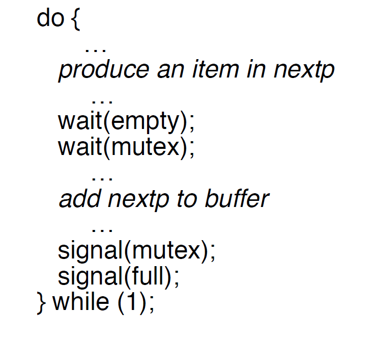
    13. Producer-Consumer Problem
    • Problem
      • The bounded-buffer producer-consumer problem assumes there is a buffer of size n
      • The producer process puts items to the buffer area
      • The consumer process consumes items from the buffer
      • The producer and the consumer execute concurrently
    • Make sure that
      • the producer and the consumer do not access the buffer area and related variables at the same time
      • no item is made available to the consumer if all the buffer slots are empty
      • no slots in the buffer is made available to the producer if all the buffer slots are full
    • Shared data
      • semaphore full, empty, mutex
    • Initially
      • full = 0; //the number of full buffers
      • empty = n; //the number of empty buffers
      • mutex = 1; // semaphore controlling the access to the buffer pool
    • Producer Process
    • Consumer Process

    14. Readers-Writers Problem

    • Problem
      • A data object( e.g. a file) is to be shared among several concurrent processes
      • A write process must have exclusive access to the data object
      • Multiple reader processes may access the shared data simultaneously without a problem
    • Shared data
      • semaphore mutex, wrt
      • int readaccount
    • Initially
      • mutex = 1
      • readcount = 0, wrt= 1
    • Writer Process
    • Read Process
    15. Dining-Philosophers Problem
    • Problem
      • five phisolophers share a common circular table
      • there are five chopsticks and a bowl of rice (in the middle)
      • when a philosopher gets hungry, he tries to pick up the closest chopsticks
      • a philosopher may pick up only one chopstick at a time, and he cannot pick up one that is already in use. 
      • when done, he puts down both of his chopsticks, one after the other.
    • Shared Data
      • semaphore chopsticks [5]
    • Initially
      • all semaphore values are 1

    Thread

    1. Definition

    • Idea: allow multiple thread of execution within the same process environment, to a large degree independent of each other.
    • Multiple threads running in parallel in one process is analogous to having multiple processes running in parallel in one computer.
    • Multiple threads within a process will share 
      • the address space
      • open files
      • other resources
    • Potential for efficient and close cooperation
    2. Multithreading
    • when a multithread process is run on a single CPU system, the threads take turns running
    • All threads in the process have exactly the same address space
    • each thread can be in any one of the several states, just like processes
    • Each thread has its own stack
    3. Benefits
    • Responsiveness
      • multithreading an interactive application may allow a program to continue running even if part of it is blocked or performing a lengthy operation
    • Resource sharing
      • sharing the address space and other resources may result in high degree of cooperation
    • Economy
      • creating/managing processes is much more time consuming than managing threads
    • Better utilization of multiprocessor architectures
    4. Example: a multi-threaded web server
    5. Implementing threads
    • processes usually start with a single thread
    • usually, library procedures are invoked to manage threads
      • thread_create: typically specifies the name of the procedure for the new thread to run
      • thread_exit
      • thread_join: blocks the calling thread until another (specific) thread has exited
      • thread_yield: voluntarily gives up the CPU to let another thread run
    • threads may be implemented in the user space or in the kernel space
    6. User-level thread
    • user threads are supported above the kernel and are implemented by a thread library at the user level
    • the library (or run-time system) provides support for thread creation, scheduling and management with no support from the kernel
    • when threads are managed in user space, each process needs its own private thread table to keep track of the threads in that process
    •  the thread-table keeps track only of the per-thread items (program counter, stack pointer, register, state…)
    • when a thread does something that may cause it to be blocked locally (e.g., wait for another thread), it calls a run time system procedure
    • if the thread must be put into blocked state, the procedure performs switching
    7. User-level advantage
    • the operating system does not need to support multi-threading
    • since the kernel is not involved, thread switching may be very fast
    • each process may have its own customized thread scheduling algorithm
    • thread scheduler may be implemented in the user space very efficiently
    8. User-level threads: problems
    • the implementation of blocking system calls is highly problematic (e.g., read from the keyboard). All the threads in the process risk being blocked
    • Possible solutions
      • change all system-call to non-blocking
      • sometimes it may be possible to tell in advance if a call will block (e.g., select system call in some version of unix) 
        • jacket code round system calls
    9. Kernel-level threads
    • kernel threads are supported directly by the OS
      • the kernel provide threat creation, scheduling and management in the kernel space
    • the kernel has a thread table that keeps track of all threads in the system
    • all calls that might block a thread are implemented as system call (at greater cost)
    • when a thread blocks, the kernel may choose another thread from the same process, or a thread from a different process
    10. Hybrid Implementation
    • An alternative solution is to user kernel-level threads, and then multiplex user-level threads onto some or all of the kernel threads
    • A kernel-level thread has some set of user-level threads that take turns using it

    11. Windows XP threads
    • windows XP support kernel-level threads
    • the primary data structures of a thread are 
      • ETHREAD (executive thread blocks)
        • thread start address
        • pointer to parent process
        • pointer to corresponding KTHREAD
      • KTHREAD (kernel thread block)
        • scheduling and synchronizing information
        • kernel stack (used when the thread is running in kernel mode)
        • pointer to TEB
      • TEB (thread environment block)
        • thread identifier
        • user-mode stack
        • thread-local storage
    12. Linux Threads
    • In addition to fork() system call, Linux provides the clone() system call, which may be used to create threads
    • Linux users the term task (rather than process or thread) when referring to a flow of control
    • A set of flags, passed as arguments to the clone() system call determine how much sharing is involved (e.g., open files, memory space, etc).

    Process Communication

    1. Process Communication

    • Mechanism for processes to communicate and to synchronize their actions
    • Two models
      • communication through a shared memory
      • communication through message passing

    2. Communication through message passing

    • Message system
      • processes communicate with each other without resorting to shared variables
      • A message passing facility must provide at least two operations
        • send(message, recipient)
        • receive(message, recipient)
      • with indirect communication, the message are sent to and received from mailboxes
    • Messaging passing can be either blocking (synchronous) or non-blocking (asynchronous)
      • blocking send: the sending process is blocked until the message is received by the receiving process or by the mail box
      • non-blocking send: the sending process resumes the operation as soon as the message is received by the kernel
      • blocking receive: the receiver blocks until the message is available
      • non-blocking receive: receive operation does not block, it either returns a valid message or a default value (null) to indicate a non-existing message
    3. Communication through shared memory
    • The memory region to be shared must be explicitly defined
    • using system calls, in unix
      • shmget: creates a shared memory block
      • shmat: maps an existing shared memory block into a process’s address space
      • shmdt: removes (unmaps) a shared memory block from the process’s address space
      • shmctl: is a general-purpose function allowing various operations on the shared block (receive information about the block, set the permissions, lock in memory)
    • Problems with simultaneous access to the shared variables
    • Compilers for concurrent programming languages can provider direct support when declaring variables.

    Virtual Machine

    1. Virtual Machines

    • Originally proposed and implemented for VM Operating System (IBM)
    • A virtual machine provides an interface identical to the underlying bare hardware
    • Each user is given its own virtual machine
    • The operating system creates the illusion of multiple processes, each executing on its sown processor with its own (virtual) memory