logic expression conversion in ILP
Reply

 balls, then the probability that each bin in C has at least one ball is at most
  if
if  , where
  is some constant strictly less than 1. If
  , then the probability is at most
  .
.
Comment: conpon analysis + chernoff bound
 , then the probability that there are at most
  occupied bins is at most
  .
. of the bins in
  have at least one ball is at most
  if
if  ; and at most
  if
if  .
. [1] Co-Location-Resistant Clouds, by Yossi Azar et al. in CCSW 2014
If there are n candidates, and we do not want to interview all candidates to find the best one. We also do not wish to hire and fire as we find better and better candidates.
Instead, we are willing to settle for a candidate who is close to the best, in exchange of hiring exactly once.
For each interview we must either immediately offer the position to the applicant or immediately reject the applicant.
What is the trade-off between minimizing the amount of interviewing and maximizing the quality of the candidate hired?
We analysis in the following to determine the best value of k that maximize the probability we hire the best candidate. In the analysis, we assume the index starts with 1 (rather than 0 as shown in the code).
Let  be the event that the best candidate is the
  -th candidate.
Let  be the event that none of the candidate in position
  to
to  is chosen.
Let  be the event that we hire the best candidate when the best candidate is in the -th position.
We have  since and are independent events.


Setting this derivative equal to 0, we see that we maximize the probability, i.e., when  , we have the probability at least
  .
.
Reference
[1] Introduction to Algorithms, CLSR
参开资料:
http://www.zhihu.com/question/23527615
随机过程一般理论
– 概率论、随机过程的测度论基础:probability space、convergence theory、limit theory、martingale theory
– Markov process
– stochastic integral
– stochastic differential equations
– semimartingale theory
数学金融:
– stochastic integrals
– stochastic differential equations (SDE)
– semimartingale
– Ito process
– Levy process: 解决ruin问题
– Brownian motion
 be the n-th renewal
 = time of the last renewal (prior to time t)
 is called the age of the renewal process
 ?
?  is the area under the curve for one cycle
![E(R_n)) = E[(X_n)^2/2] = E[X^2_n]/2](http://mytechroad.com/wp-content/ql-cache/quicklatex.com-e4d688a2d68c2f419a78f8b28779c786_l3.png "Rendered by QuickLaTeX.com")
![frac{E[R_n]}{E[X_n]} = frac{E[X^2_n]}{2E[X_n]}](http://mytechroad.com/wp-content/ql-cache/quicklatex.com-359d1e6c78190b06e998d4f715968a63_l3.png "Rendered by QuickLaTeX.com")

 be a renewal process = reward earned at
  -th renewal are i.i.d, but can depend on
  (length of the -th cycle)
 is a renewal reward process.
 = cumulative reward earned up to time t
![lim_{t to infty} frac{R(t)}{t} = frac{E[R_n]}{E[X_n]}](http://mytechroad.com/wp-content/ql-cache/quicklatex.com-44cb2a0abc58e69e0f04ad6b0ca3aca2_l3.png "Rendered by QuickLaTeX.com")
![lim_{t to infty} frac{E[R(t)]}{t} = frac{E[R_n]}{E[X_n]}](http://mytechroad.com/wp-content/ql-cache/quicklatex.com-4c18a20cfab623eed5844ba13ab551e6_l3.png "Rendered by QuickLaTeX.com")
![E[R_n] < infty, E[X_n] < infty](http://mytechroad.com/wp-content/ql-cache/quicklatex.com-716232bf33db1f64213028da321af8c2_l3.png "Rendered by QuickLaTeX.com")
Problem:

Solution:

Let  be a Markov chain with transition probabilities
  .
.

E.g. A sample realization is 1, 2, 3, 4, 5
Let  be the same sequence in reverse, i.e.
Let  be the transition probabilities of the reversed process. That is
= 
= 
= 
In the steady state, assuming the limiting probabilities exist, we have or
or 
The above equation is saying that the rate of transmissions from i to j in the reversed chain is equal to the rate of transitions from j to i in the forward chain.
A DTMC is time reversible if 
– Stochastic Course Notes
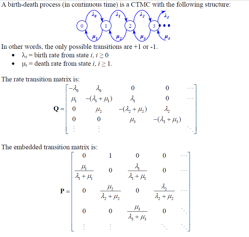


– Stochastic Course Notes
Consider a population
 . Key assumption: This distribution is constant over time.
 for all j (i.e., the problem is not deterministic) be the size of the population at period n

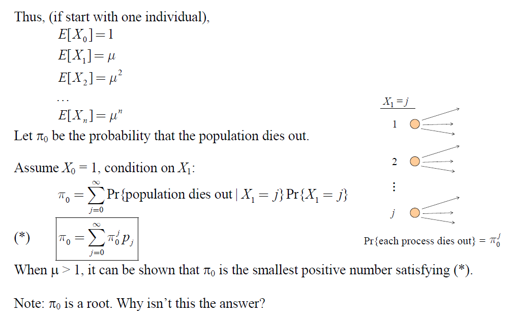

Problem:

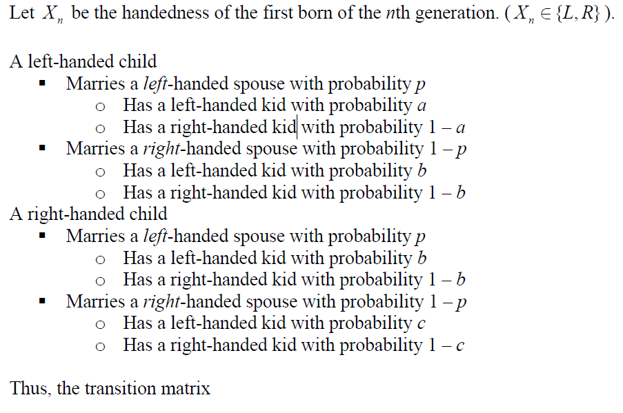
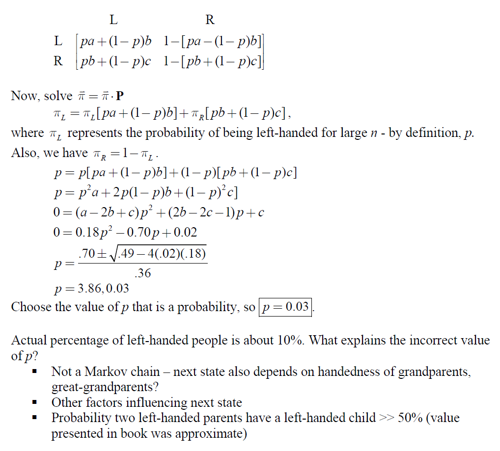
– Stochastic Process Course Notes
Problem:

Solution:


