[Stochastic Process] Black-Scholes Formula

Posted on November 27, 2014 by admin

1. Introduction

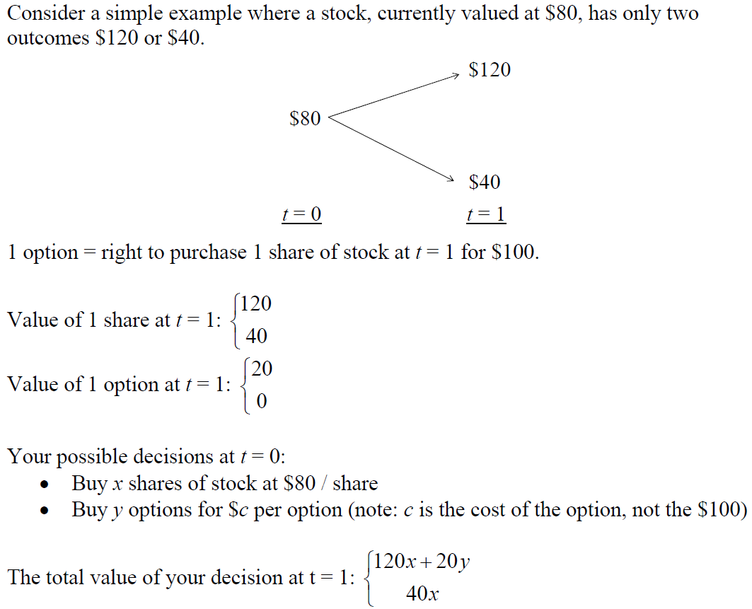
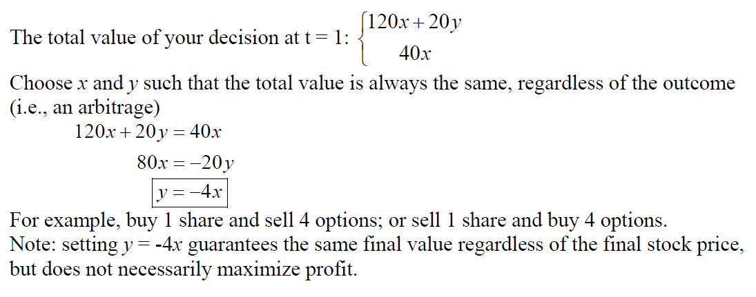
Motivation: Find the cost of buying options to prevent arbitrage opportunity.

Definition: Let $x(s)$ be the price of a stock at time s, considered on a time horizon $s in [0,t]$ . The following actions are available:

At any time s, $0 leq s leq t$ , you can buy or sell shares of stock for $X(s)$
At time $s = 0$ , there are N options available. The cost of option $i$ is $c_i$ per option which allows you to purchase $1$ share at time $t_i$ for price $k_i$ .

Objective: the goal is to determine $c_i$ so that no arbitrage opportunity exists.

Approach: By the arbitrage theorem, this requires finding a probability measure so that each bet has zero expected pay off.

We try the following probability measure on $X(t)$ : suppose that $X(t)$ is geometric Brownian motion. That is, $X(t) = x_0 e^Y(t)$ , where $Y(t) = sigma B(t) + mu t$ .

2. Analyze Bet 0: Purchase 1 share of stock at time s

Now, we consider a discount factor $alpha$ . Then, the expected present value of the stock at time t is

$E[e^{-alpha t} X(t) | X(s)] = e^{-alpha t} X(s) e { mu/(t-s) + frac{sigma^2(t-s)}{2}}$

Choose $mu, sigma$ such that $alpha = mu + sigma^2/2$

Then $E[e^{-alpha t} X(t) | X(s)] = e^{-alpha t} X(s) e^{-alpha(t-s)} = e^{-alpha s} X(s)$ .

Thus the expected present value of the stock at t equals the present value of the stock when it is purchased at time s. That is, the discount rate exactly equals to the expected rate of the stock returns.

3. Analyze Bet i: Purchase 1 share of option i (at time s =0)

First, we drop the subscript i to simplify notation.

Expected present value of the return on this bet is

$- c + E[max (e^{alpha t} X(t)- k), 0]$
= $-c + E[e^{-alpha t} (X(t) - k)^+]$

Setting this equal to zero implies that
$ce^{alpha t} = E[ (X(t) - k)^+] = E[(x_0 e^{Y(t)} - k)^+]$
= $int^{infty}_{-infty} (x_0 e^y - k)^+ frac{1}{2 pi sigma^2 t} e^{-frac{(y-ut)^2}{2 sigma^2 t}} dy$

$(x_0 e^y - k)+$ has value 0 when $x_0 e^{Y(t)} - k leq 0$ , i.e., when $Y(t) leq ln(k/x_0)$

Thus the integral becomes
$ce^{alpha t} = E[ (X(t) - k)^+] = E[(x_0 e^{Y(t)} - k)^+]$
= $int^{infty}_{ln k/x_0} (x_0 e^y - k)^+ frac{1}{2 pi sigma^2 t} e^{-frac{(y-ut)^2}{2 sigma^2 t}} dy$

Now, apply a change of variables:
$w = frac{y - mu t}{sigma sqrt(t)}$ , i.e., $</span>sigma sqrt(t) w + mu t = y$

4. Summary

No arbitrage exists if we find costs and a probability distribution such that expected outcome of every bet is 0.

If we suppose that the stock price follow geometric Brownian motion and we choose the option costs according to the above formula, then the expected outcome of every bet is 0.
Note: the stock price does not actually need to follow geometric Brownian motion. We are saying that if stock price follow Brownian motion, then the expected outcome of very bet would be 0, so no arbitrage exists.

A few sanity checks

When $t = infty$ , cost of option is $x_0$
When $t=0$ , cost of option is $x_0 - k$
As t increases, c increases
As k increases, c decreases
As $x_0$ increases, c increases
As $sigma$ increase, c increase (assuming $mu >0$ )
As $alpha increases$ , c decreases

[Stochastic Process] Arbitrage

Posted on November 26, 2014 by admin

1. Introduction

Definition: the simultaneous buying and selling of securities, currency, or commodities in different markets or in derivative forms in order to take advantage of differing prices for the same asset.

2. Option Pricing

Question:

How to choose x and y:

How to maximize profit:

Key Assumption: There is no limit to buying or selling of options. In practice,

you may only be able to buy, but no sell, for example.

3. Aibitrage Theorem

Definition:
Consider n possible wagers ${1,2, cdots, n}$ on m possible outcomes: ${1,2,cdots, m}$ .
Let $r_i(j)$ to be the outcome of wagers i if outcome j occurs.
If $X_i$ is bet on wager $i$ , then $x_i r_i(j)$ is earned if outcome j occurs.

Arbitrage Theorem:

$exists vec{p}$ such that $sum^m_{j=1} p_j r_i(j) = 0$ , $forall i$
$exists vec{x}$ such that $sum^n_{i=1} x_i r_i(j) > 0$

Intuitively,

First theorem: there is a probability vector such that the expected outcome of every bet is 0, or
There existing a betting scheme that leads to a sure win.

## TODO: explain more about these two theorem

[Stochastic Process] Geometric Brownian Motion

Posted on November 26, 2014 by admin

1. Motivation

Definition: Let $X(t)$ be Brownian motion with drift coefficient $mu$ and variance parameter $sigma^2$ . Let $Y(t) = e^{-X(t)}$ . Then $Y(t)$ is geometric Brownian motion.

Motivation: Let $Y(_n)$ be the price of a stock at time $n$ (where n is distance); Let $X(n) = frac{Y_n}{Y_+{n-1}}$ be the fractional increase/decrease in the price of the stock from time n-1 to time n.
We suppose that $X_n$ are i.i.d. Then
$Y_n = X_n Y_{n-1} = X_n X_{n-1} X_{n-1} cdots X_1 Y_0$
$ln Y_n = ln X_n X_{n-1} X_{n-1} cdots X_1 Y_0 = ln Y_0 + sum^n_{i=1} ln X_i$

The process $ln(Y_n)$ looks like a random walk.

2. Property of Geometric Brownian Motion

$E[Y(t) | Y(s) = y_s] = y_s E[e^{{X(t) - X(s)}}]$

Proof: $E[Y(t) | Y(s) = y_s] = E[e^{X(t)} | X(s) = ln y_s]$

= $E[e^{X(t) - X(s) + X(s)} | X(s) = ln y_s]$

= $y_s E[e^{X(t) - X(s)}]$

E[Y(t) | Y(s) = y_s] = y_s e^{mu(t-s) + sigma^2(t-s)/2}

Proof: If W ~ $N(mu, sigma^2)$ , then $e^W$ is lognormal with mean $E[e^W] = e^{mu + sigma^2/2}$
Thus, {X(t) – X(s)} ~ $N[mu(t-s), sigma^2(t-s)]$ , since $X(t)$ is Brownian motion with drift

Note: if $mu = 0$ , then $E[Y(t)|Y(0) = y_0 ] = y_0 e^{sigma^2 t/2}$ . Thus $E[Y(t)]$ is increasing even though the jump process with $X(t)$ is symmetric

3. Example
Question: You invest 1000 dollars in the stock market. Suppose that the stock market can be modeled using geometric Brownian motion with an average daily return of 0.03% and a standard deviation of 1.02%. what is the probability that your money increases after 1 year (260 business days?) 10 years? 30 years?

Answer: Let $X(t) = mu t + sigma B(t)$ , where $B(t)$ is standard Brownian Motion.
Let $Y(t) = Y_0 e^{X(t)}$ where $B(t)$ is standard Brownian motion, $X(t)$ is Brownian motion with drift, and $Y(t)$ is geometric Brownian motion.

$Pr(Y(t) > Y_0) = Pr(Y_0 e^{X(t)} > Y_0)$
= $Pr(e^{X(t)} > 1)$
= $Pr(X(t) > ln 1 = 0)$
= $Pr(N(mu t, sigma^2 t) > 0)$
= $1 - Phi(frac{-mu t}{sigma sqrt{t}})$
= $Phi(frac{mu sqrt{t}}{sigma})$

[Stochastic Process] Brownian Motion

Posted on November 25, 2014 by admin

Course notes for “Stochastic Process”

2014 Fall

1. Motivation

Brownian motion can be thought of a symmetric random walk where the jumps sizes are very small and where jumps occur very frequently.

Each jump size are $Delta x$
The time before two jumps are $Delta t$ .

1.1 What’s the mean and variance?

Let $X_i$ denote whether the i-th jump is to the right(+1) or to the left(-1), we have $X_i =1, -1$ with probability $frac{1}{2}$ and $frac{1}{2}$ respectively.
Thus, $E[X_i] = 0$ and $Var[X_i] = E[X^2_i] - E[X_i]^2 = 1$ .

Let $X$ denote the state of Markov Chain after n jumps, then
$X = Delta x cdot (X_1+X_2+cdots+X_n)$
The $X(t)$ denote the continuous Markov Chain after n jumps, then
$X(t) = Delta x cdot (X_1 + X_2 + cdots + X_{|t/Delta t|})$

Then we have
$E[X(t)] = 0$ and $Var[X(t)] = (Delta x)^2 cdot frac{t}{Delta t}$ .

Let $Delta x = sigma sqrt{Delta t} to 0$ , then
$V[X(t)] = (Delta x)^2 cdot frac{t}{Delta} to sigma^2 t$ .

2. Properties of Brownian Motion

(1) $X(0) = 0$
(2) $X(t) ~ N(0, sigma^2 t)$
(3) X(t) has independent increments
i.e., $X(t_2) - X(t_1)$ is independent of $X(t_4) - X(t_3)$ assuming the intervals of $[t_1,t_2]$ and $[t_3,t_4]$ are disjoint.
(4) X(t) has stationary increments
i.e., $X(t_2) - X(t_1)$ has the same distribution as $X(t_4) - X(t_3)$ if $t_2 - t_1 = t_4 - t_3$ .

Example: What’s the distribution of $X(t_2) - X(t_1)$ ?

Answer: by the stationary property, we have $X(t_2) - X(t_1)$ ~ $N(0, sigma^2(t_2 - t_1))$ .

3. Standard Brownian Motion (SBM)

SBM ~ $N(0,1)$
Let $Y(t) = frac{X(t)}{sigma} = sqrt{Delta t}$ , then $V[Y(t)] = 1$ .

4. Brownian Motion with Drift

Definition 1: Let $B(t)$ be the standard Brownian motion. Let $X(t) = sigma B(t) + mu t$ , then $X(t)$ is Brownian motion with drift $mu$ .

Definition 2: ${X(t); tge 0}$ . $X(t)$ is Brownian Motion with drift $mu$ and variance parameter $sigma^2$ if

$X(0) = 0$
${X(t); t geq 0}$ has stationary and independent increments
$X(t)$ ~ $N(mu t , sigma^2 t)$

Example: Let $X(t)$ be Brownian motion with $sigma = 2$ and drift $mu = 0.1$ . What is $Pr{X(30) >0 | X(10) = -3}<u>Answer: </u>$ Pr{X(30) >0 | X(10) = -3} $=$ Pr{X(30) – X(20) >3 | X(10) =3 } $=$ Pr{X(30) – X(10) >3 } $(independent property) =$ Pr{X(20) – X(0) >3 } $(stationary property) =$ Pr{X(20)>3 } $(X(0) = 0) =$ Pr{N(2,80) > 3} = Pr{X(0,1) > frac{3-2}{sqrt{80}} $=$ 1-Phi(frac{1}{4sqrt{5}}) $.<b><span style="font-size: x-large;">5. Brownian Bridge</span></b><b><u>Basic Idea:</u> </b>condition on the final value of a Brownian motion process and derive the stochastic properties in between.<u style="font-weight: bold;">Main Results </u>:$ X(s) = x | X(t) = B $is normally distributed with<ul><li><span style="color: red;">Mean:$ frac{s}{t} cdot B $</span></li><li><span style="color: red;">Variance:$ frac{s}{t} cdot (t-s) $</span></li><li>The value of s with the highest variance is$ s = t/2 $. That is, we know the endpoints of the process, but we don't know exactly what happens in between.</li></ul><b>Note</b>: these results are for standard Brownian motion (SBM)<b><u>Proof:</u></b><div style="clear: both; text-align: center;"><a href="http://2.bp.blogspot.com/-fYCRQBP77lY/VHVa9KUoD4I/AAAAAAAAAUs/CDAwrhLMdK8/s1600/BMBridgeProof.PNG" style="margin-left: 1em; margin-right: 1em;"><img border="0" src="http://2.bp.blogspot.com/-fYCRQBP77lY/VHVa9KUoD4I/AAAAAAAAAUs/CDAwrhLMdK8/s1600/BMBridgeProof.PNG" height="640" width="528" /></a></div><div style="clear: both; text-align: center;"></div><div style="clear: both; text-align: left;"></div><div style="clear: both; text-align: left;"><u style="font-weight: bold;">Example 1: </u>Suppose you have a stock whose value follows Brownian motion with$ X(t) $~$ N(0, sigma^2 t) $. If the stock is up$ 10 after 6 hours, what is the probability that the stack was above its starting value after 3 hours?

Answer: $Pr ( X(3) > 0 | X(6) = 10 ) = P( sigma cdot Y(3) >0 | sigma cdot Y(6) = 10) = P( Y(3) > 0 | Y(6) = 2.5$

This is a Brownian bridge process where $(Y(3) | Y(6) = 2.5)$ ~ $N(3/6 cdot 2.5, 3 cdot 6 cdot 3)$ = $N(5/4, 3/2)$ .

Thus $P( Y(3) > 0 | Y(6) = 2.5) = P(N(1.25,1.5) > 0$

Example 2: If a bicycle race between two competitors, Let $X(t)$ denote the amount of time (in seconds) by which the racer that started in the insider position is ahead when 100t percent of the race has been completed, and suppose that $X(t), 0 leq t leq 1$ , can be effectively modeled as a Brownian Motion process with variance parameter $sigma^2$ .

6. First Passage Time

Let $T_a$ denote the first time that standard Brownian motion hits level a (starting at X(0) = 0), assuming a >0, then we have
$Pr{X(t) geq a} = Pr{X(t) geq a | T_a leq t} cdot Pr{T_a leq t} + Pr{X(t) geq a | T_a > t}Pr{T_a geq t}$

$Pr{X(t) geq a | T_a leq t} = frac{1}{2}$ : you know that at some time before t, the process hits a. From that point forward, you are just as likely to be above a as below a.
$Pr{X(t) geq a | T_a > t} = 0$ : $X(t)$ cannot be above a, because the first passage time to a is after t.

Thus, $Pr{X(t) geq a} = frac{1}{2} Pr{T_a leq t}$ ,

$Pr{T_a leq t} = 2 Pr{ X(t) geq a} = frac{2}{sqrt{2pi t}} int^infty_{a} e^{-x^2/2t} dx$ .

Change variables: $y = frac{x}{sqrt{t}}$ , we have $Pr{T_a leq t} = frac{2}{sqrt{2pi}} int^infty_{a/sqrt{t}} e^{-y^2/2t} dy$ .
By symmetry, we get $Pr{T_a leq t}$ .

Lisa Tech Blog

My security road

Monthly Archives: November 2014